Review

The returns R(t) is taken as a stochastic process indexed by the time parameter, which is generally assumed to be stationary for the purpose of any kind of predictive capability. Stationarity means that the probability that R(t) takes values in a set B does not change with time t.

Additional assumptions are imposed based on the need and appropriateness. The most common additional assumption is normality of the distribution in which case the mean and the variance are estimated from a sample data and used for the purposes of prediction etc.,

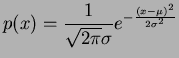
The reason of the assumption of normality is the central limit theorem which says that a sum of independent and identically distributed random variable each having finite variance (suitably normalized) will converge to a random variable which is normally distributed. The normal (or the Gaussian) distribution is one whose probability density function is given by

$$p(x) = \frac{1}{\sqrt{2\pi}\sigma}e^{-\frac{(x-\mu)^2}{2\sigma^2}}$$

where the mean is $\mu$ and the variance is $\sigma^2$ are the parameters that determine the distribution. The Gaussian distribution has the property that if $X_1,\dots, X_n$ are i.i.d Gaussian random variables, then the random variable $\sum_{i=1}^n X_i$ also has a Gaussian distribution (though with a different variance). This shows a stability of the form of the distribution under taking sums.

On the other hand in the recent past it has been discovered in several international markets [1] that the distribution of returns is not necessarily Gaussian, but is fat tailed (meaning that it does not have rapid decay as $x \rightarrow \infty$) and behaves like

$$p_{\alpha}(x) \approx C x^{-\alpha} ~~~$$   as$$~~~ \vert x\vert \rightarrow \infty$$

for some $1<\alpha < 2$. It is also discovered that the $p_\alpha(x)$ has the property that the sum of random variables with the above distribution $p_\alpha(x)$ also have a distribution with a similar form. The class that are considered in the literature are Levy stable ones, that is those $p(x)$ with the property that their Fourier transform

$$\widehat{p}(k) = \int_{-\infty}^{\infty} p(x) ~ e^{-ikx} ~ dx$$

looks like a multiple of $e^{-\vert k\vert^\beta}$ for some $1< \beta < 2$ (to compare with the normal distribution recall that the Fourier transform of the normal distribution looks like a multiple of $e^{2\sigma^2(k)^2}$).

The model valid for a given market is important to determine the VaR valid for that market. The model building can be done in several ways. One could assume that the distribution $p(x)$ valid for a market has one of the above forms and then go about deciding the parameters of the model or simply build the model using the relative frequency definition for the distribution $p(x)$, which is the number of times the value $x$ is taken to the total number of observations (also known broadly as Historical Simulation).

In all the above we should remember that there is still the assumption of stationarity of the returns over time.