LECTURE VIII
OTHER SURFACES
KAPIL HARI PARANJAPE
An irreducible projective variety S of dimension 2 is called a projective surface.
One way to study surfaces is to think of them as “moving curves” with one parameter. More precisely, we
can ask for a curve C and an irreducible closed subvariety (which we can think of as a correspondence)
T ⊂ C ×S such that the fibre over each point of C is a curve in S. We have already seen one such example,
that of ruled surfaces in the previous section. Going on from there it is natural to take up the
study of surfaces where a C and T can be found where the (general) fibre is a curve of genus
1.
A different way to approach the study of surfaces is to extend our knowledge of plane curves and study
surfaces in ℙ3 or equivalently sub-varieties of ℙ3 defined as the vanishing locus of a single irreducible
homogeneous polynomial F(W,X,Y,Z).
One may also try to generalise the Riemann-Hürwitz approach by thinking of surfaces given in the form
of a finite morphism S → ℙ2. In the case of curves given as C → ℙ1 the topology is rather simply described
as the branch locus is a finite set of points in ℙ1. However, the situation of surfaces is made more
complicated by the numerous types of curves in ℙ2. As a result this approach is much more
difficult.
Let us thus begin with surfaces in ℙ3. We have already studied the surfaces in ℙ3 defined by equations of
degree 2, so let us continue with surfaces of degree 3. We will show that a smooth cubic surface S in ℙ3 has
27 lines which are in a rather special position with respect to each other and contain a configuration known
as the “Schlafly double-six”. Before we do that let us take the projection of S from a general line M in ℙ3.
We obtain a morphism S \ S ∩ M → ℙ1 where S ∩ M consists of 3 distinct points. Let  be the
closure of the graph of this morphism. As seen earlier the fibre Ei of
be the
closure of the graph of this morphism. As seen earlier the fibre Ei of  → S over a point i in
S ∩ M consists of a copy of ℙ1 which can be identified with the projective space of directions
tangent to S at i. Moreover, each of these copies is mapped isomorphically under the natural map
π :
→ S over a point i in
S ∩ M consists of a copy of ℙ1 which can be identified with the projective space of directions
tangent to S at i. Moreover, each of these copies is mapped isomorphically under the natural map
π :  → ℙ1. Each fibre of π is a plane cubic curve; we have seen that this is a curve of genus 1.
Thus the study of the cubic surface generalises the study of ruled surfaces as well. An easy
exercise in computing the degree of the dual variety shows that if M is a general line (and the
characteristic is zero), then there are exactly 6 singular fibres and each such fibre is a nodal
plane cubic. The following study of the cubic surface can therefore be interpreted in terms of
the group structure on the generic fibre of π; those interested may try to follow this approach
later.
→ ℙ1. Each fibre of π is a plane cubic curve; we have seen that this is a curve of genus 1.
Thus the study of the cubic surface generalises the study of ruled surfaces as well. An easy
exercise in computing the degree of the dual variety shows that if M is a general line (and the
characteristic is zero), then there are exactly 6 singular fibres and each such fibre is a nodal
plane cubic. The following study of the cubic surface can therefore be interpreted in terms of
the group structure on the generic fibre of π; those interested may try to follow this approach
later.
We first show that there is one cubic surface which has exactly 27 lines. To begin with let us choose a
smooth cubic surface S that contains a line L; for example we can take the surface defined by the equation
WX(W - X) = Y Z(Y - Z) which contains the line defined by W = Y = 0. More generally, the surface
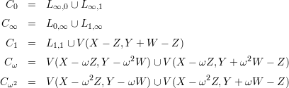
S0 and contains the lines La,b which are defined by the equations W - aX = 0 Y - bZ = 0
where (a,b) run over the set {0,1,∞}2. The projection of S0 from the line L∞,∞ is given by the
morphism

which clearly extends to a morphism f : S0 → ℙ1. The fibre of f over the point (t : 1) of ℙ1 is the conic Ct
defined by Y (Y -Z) = tW(W -tZ) in the plane defined by X = tZ. This conic becomes a pair of straight
lines for t in the set {0,∞,1,ω,ω2} where ω is a primitive cube root of 1; this gives all the
lines that are contained in the fibres of f or equivalently all lines that meet L∞,∞. We have
The line L0,0 meets only the following 5 lines from amongst these: N1 = L∞,0, N2 = L0,∞, N3 = L1,1,
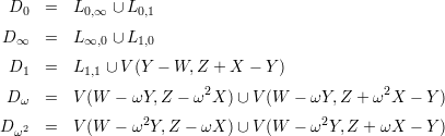
N4 = V (X - ωZ,Y - ω2W), N5 = V (X - ω2Z,Y - ωW). Interchanging W with X and Y with X we
see that the pairs of lines Dt defined as follows give precisely all lines in S0 that meet L0,0:
We see that the 5 lines Ni listed previously are the only lines that meet both L0,0 and L∞,∞.
Now consider the union Qijk of the locus of all lines that meet Ni, Nj, Nk for some triple
{i,j,k} contained in {1,2,3,4,5}. As seen earlier this surface Qijk is a smooth quadric surface
which has two rules, one given by the lines that meet Ni, Nj and Nk and another ruling that
contains these lines. In particular, the intersection of Qijk and S0 is a degree 6 locus and must
consist of 3 lines from the first ruling; L0,0 and L∞,∞ give two such lines and we obtain one
more which we call Mijk. Conversely, given a line M inside S which does not meet L0,0 or
L∞,∞, we can form a quadric Q that is the union of all lines meeting L0,0, L∞,∞ and M. The
intersection of Q and S is of degree 6 and contains these lines; thus it consists of exactly 3
lines out of the Ni’s. We now see that we have  = 10 lines M that are skew to each of L0,0
and L∞,∞. Combining the above calculations we see that we have 9 + 5 + (5 - 2) + 10 = 27
lines.
= 10 lines M that are skew to each of L0,0
and L∞,∞. Combining the above calculations we see that we have 9 + 5 + (5 - 2) + 10 = 27
lines.
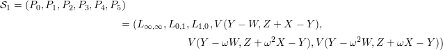
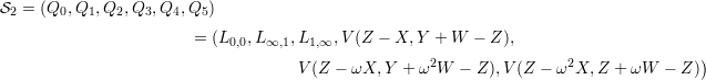
The following combinatorial description helps us to identify this as a “double-six”. Consider the 6-tuples
and
We
observe that each of these 6-tuples consists of mutually disjoint lines. We have already noted that P0
(respectively Q0) meets each of the lines Qi (respectively Pi) for i 0. Consider the line P1. The span of P1
and Q0 is a plane that contains N1. So P1 meets N1 which lies in the plane spanned by P0 and Q1.
On the other hand P1 is disjoint from the line Ni for i
0. Consider the line P1. The span of P1
and Q0 is a plane that contains N1. So P1 meets N1 which lies in the plane spanned by P0 and Q1.
On the other hand P1 is disjoint from the line Ni for i 1 and from the line P0. The plane
spanned by these contains the line Qi and so P1 must meet it. In other words, P1 meets all the
elements of
1 and from the line P0. The plane
spanned by these contains the line Qi and so P1 must meet it. In other words, P1 meets all the
elements of  2 \{Q1}. Similarly, we can show that Pi meets all the elements of 2 \{Qi} for other
i.
2 \{Q1}. Similarly, we can show that Pi meets all the elements of 2 \{Qi} for other
i.
A double-six consists of a pair of ordered 6-tuples of lines (P0,…,P6) and (Q0,…,Q6)
such that each Pi meets all the Qj except Qi.
Now, for each i and j Consider the intersection of the plane spanned by Pi and Qj with that spanned by Pj
and Qi; this gives a line Rij which meets all the four lines. In the previous terminology we have
R0i = Ni and Rlm = Mijk where {i,j,k,l,m} = {1,2,3,4,5}. This gives us 6 + 6 +  = 27
lines.
= 27
lines.
The projective space of dimension  - 1 = 19 parametrises all homogeneous cubic polynomials in 4
variables or equivalently cubic surfaces in ℙ3. As we have seen before there is a 4 dimensional variety
𝔾(1, ℙ3) that parametrises lines in ℙ3. Let I denote the sub-variety of ℙ19 × 𝔾(1, ℙ3) that consists of pairs
(S,L) such that L is contained in S. For each L we obtain 4 linear conditions which are the equations that
define the locus of cubics that contain L. In other words the fibre of I over each point of 𝔾(1, ℙ3) is a linear
ℙ15 in ℙ19; so I is also 19-dimensional. We have shown that the fibre of I → ℙ19 consists of finitely many
points over the point corresponding to the surface S0. It follows that this is a surjective morphism. In
particular, each cubic surface contains a line. One can then duplicate the argument given above
to show that the configuration of lines in the cubic form is generated from the “double-six”
as described above. (Warning: There could be some additional incidence conditions in some
cases. When three lines among the 27 lie in a plane then they may form a “star” instead of a
“triangle”.)
- 1 = 19 parametrises all homogeneous cubic polynomials in 4
variables or equivalently cubic surfaces in ℙ3. As we have seen before there is a 4 dimensional variety
𝔾(1, ℙ3) that parametrises lines in ℙ3. Let I denote the sub-variety of ℙ19 × 𝔾(1, ℙ3) that consists of pairs
(S,L) such that L is contained in S. For each L we obtain 4 linear conditions which are the equations that
define the locus of cubics that contain L. In other words the fibre of I over each point of 𝔾(1, ℙ3) is a linear
ℙ15 in ℙ19; so I is also 19-dimensional. We have shown that the fibre of I → ℙ19 consists of finitely many
points over the point corresponding to the surface S0. It follows that this is a surjective morphism. In
particular, each cubic surface contains a line. One can then duplicate the argument given above
to show that the configuration of lines in the cubic form is generated from the “double-six”
as described above. (Warning: There could be some additional incidence conditions in some
cases. When three lines among the 27 lie in a plane then they may form a “star” instead of a
“triangle”.)
Perhaps the first Indian mathematician in recent times who developed expertise in the study of algebraic
surfaces was C. P. Ramanujam of the TIFR. He posed some very interesting questions which
have led to a lot of research by R. V. Gurjar, A. R. Shastri and C. R. Pradeep. Their work
involves the study of surfaces which occur as genus 1 fibres over curves; this was initiated by K.
Kodaira. Such surfaces have also been studied M. M. Nori of Mumbai University. The study of
singular surfaces (or surface singularities) is where V. Srinivas of TIFR has made significant
contributions. Kodaira had classified surfaces according to their invariants much as curves are classified
in terms of the genus. The extension of this work (to varieties of higher dimension) by Mori,
Kawamata, Kollár, Shokurov and others was an important development in the late ’80s and early
’90s. Unfortunately, no Indian mathematician played a significant role in this development of
ideas.