
We study the “simplest” possible curves. Since we have declared them to be simple we can ask more difficult questions about them!
The same algebraic variety may come in many different guises so an interesting problem is to “recognise” algebraic varieties. Thus the curve ℙ1 also appears as the curve in ℙ2 defined by the equation XY - Z2 = 0; for that matter there is also the rational normal curve of degree d in ℙd. It is an interesting exercise to show that a non-degenerate (doesn’t lie in a hyperplane) irreducible curve of degree d in ℙd is isomorphic to ℙ1 once one is given a point on it. Thus the existence of rational points is quite important in recognising varieties. For example the curve in ℙ2 defined by X2 + Y 2 + Z2 = 0 (in characteristic different from 2) is isomorphic to the curve defined by XY = Z2 after a linear change of co-ordinates in a field where the first curve has a point.
As a consequence of the Riemann-Roch theorem for curves any smooth irreducible curve of genus 0 can be realised as a conic in ℙ2; thus, a very interesting number-theoretic question is to try to understand which non-algebraically closed fields k have the property that a conic over this field always has a point with co-ordinates in this field. As an exercise you can examine the case when k is finite.
Let us move on to curves of genus 1. Such curves come in a number of different guises. The most classical is the Tate-Weierstrass form
As usual, we will “complete” this curve to make it projective by taking the equation

which defines a curve in ℙ2; we note that (0 : 1 : 0) is a point of this curve which is sometimes called the origin and sometimes called the point at infinity.
However, a curve of genus 1 can come in a number of other guises. For example, we can increase the degree of the right-hand side in the above equation to obtain

We again need to “projectivise” which we do by considering the equation

in the homogeneous polynomial ring k[W,X,Y ] where W and X have degree 1 and Y has degree 2. Equivalently, we can make the substitutions X2 = T, WX = U and W2 = V to obtain the equation

in the homogeneous co-ordinate ring k[T,U,V,Y ]∕(U2 - TV ).
We note that the latter curve can be thought of the the curve defined by two quadratic equations Qi(T,U,V,Y ) = 0 for i = 1,2. So that is yet another guise in which curves of genus 1 appear.
In fact, unlike that case of curves of genus 0, curves of genus 1 can appear in infinitely many different guises, one for each integer n > 1. The situation becomes much simpler however, if we assume that k is algebraically closed or more simply that there is at least one point (in other words if the object of our study is not pointless!). If a smooth irreducible curve of genus 1 has as a point with co-ordinates in the field k then all these different disguises collapse and only the Weierstrass form remains. The reason is the Riemann-Roch theorem once again. An elliptic curve is defined to be a curve E of genus 1 with a chosen point o.
The Tate-Weierstrass form of the elliptic curve with the specially chosen point (0 : 1 : 0) has another special property. We will show that there is a natural commutative group law on this curve which thus becomes a projective group variety. Consider a pair of points (p,q) and (r,s) on the curve and consider the parametric line given by t(p,q) + (1 - t)(r,s) that passes through these points. Substituting this in the equation

we obtain a cubic polynomial equation f(t) = 0 with coefficients in the ring k[a1,a2,a3,a4,a6]. We further note that t = 0 and t = 1 are solutions of f(t) = 0 so that f(t)∕(t2 -t) is a linear polynomial. This gives us a solution for t which we substitute in order to obtain the point (u,v) which is the third point on the line. It is clear that the line x = u also contains the point (u,a1u + a3 -v). The group law on the curve is defined by

One has to also take the special cases where p = r into account. The appropriate formulae can be written down in those cases as well. It is probably easier to understand the group law more geometrically via Riemann-Roch. Let D be any divisor on the elliptic curve E and consider the divisor D - (deg(D) - 1)o. The latter is a divisor of degree 1. From Riemann-Roch it follows that this divisor is linear equivalent to an effective divisor of degree 1; in other words, there is a point p(D) such that D is linearly equivalent to the divisor (deg(D) - 1)o + p(D). Thus the group structure on divisors modulo linear equivalence becomes a group structure on points of E with o playing the role of identity.
Since we have an abelian group, it is natural to ask whether it has torsion subgroups for various orders. We will approach this problem from a slightly different viewpoint. Let O and I be conics. Pick a point A0 of O and pick one line L0 out of the two lines that contain A0 and are tangent to I. Let A1 be the second point of intersection of A0 with O; so L0 is one of the two lines which contain A1 and are tangent to I. Let L1 by the second tangent to I that contains A1. Clearly we can iterate this construction which leads to the following interesting property: If this construction is cyclic, then there is an n such that this construction gives a cycle of length n for all starting positions.
What is the relation of this construction with elliptic curves? Let G(X,Y,Z) be the equation for I and F(X,Y,Z) be the equation for O. Consider the curve C in ℙ3 defined by the equations
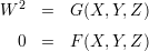
Now, the surface Q defined by the equation W2 = Y 2 - XZ has a parametric solution

This parametrisation is used to express Q in the form ℙ1 × ℙ1 where p and q represent the co-ordinates of the the point in each factor. In particular, each point Ap,q of Q determines a pair of lines Hq and V p in Q given respectively in parametric form by

The image of these lines in the (X : Y : Z) plane under projection from (W : X : Y : Z) = (1 : 0 : 0 : 0) are the lines Tq and Tp where, for each r, the line Tr
is tangent to the conic I at the point (r2 : r : 1). In fact Tp and Tq are precisely the two lines that contain the point (2pq : p + q : 2) and are tangent to the conic I. (Exercise: Carry out the above construction without the use of co-ordinates).
Now, the point Ap,q lies on the curve C if and only if its image lies on O. Conversely, given a point A0 on O and a line L0 that passes through A0 and is tangent to I, let r be such that L0 = Tr. This means that A0 = (x : y : z) = (2tr : t + r : 2), so that if we take p0 = r and q0 = (y - rz)∕z, then (x : y : z) = (2p0q0 : p0 + q0 : 2). In particular, the point Ap0,q0 maps to A0 under the above projection; note again that Ap0,q0 lies on C. We could equally well have taken the point Aq0,p0; as a convention we will pick Ap0,q0. In this case V p0 is the line in Q that maps to L0 = Tr = Tp0. Let us now follow the construction.
The line L1 is the second tangent to I from the point A0. Thus, it is the image of the line Hq0. The point A1 is the second point of intersection of L1 with the conic O; this is the image of a (unique) point Ap1,q0 that is the second intersection of Hq0 with C. Continuing this approach, we see that L2 is the image of V p1 which intersects C in the point Ap1,q1 that lies over A2. Now, we are in a position similar to the starting point and we can iterate.
It may appear that the “lifted” construction corresponds to two steps of the original construction, but note that we will consider an iteration to be complete even if we reach Aq0,p0 instead of Ap0,q0.
To see what this has to do with elliptic curves, we note that the divisors Hq ∩ C are all linearly equivalent to each other (similar story with the divisors V p ∩ C). Now consider the divisor

Treating C as an elliptic curve with the origin Ap0,q0, we can identify the divisor D with the point Ap1,q1. Note that the divisor

is linearly equivalent to D as remarked above. Thus

Thus the above iterated construction is identified with the sequence of positive integer multiples of Ap1,q1 in the group law on the elliptic curve. It is clear that the construction cycles if and only if this point is of finite order. Finally, we use the linear equivalence to again note that regardless of which point P of C we take to be the origin, the order of the point corresponding to D is the same.
The above study of a pair of quadratic forms has been taken up in depth in the work of U. Bhosle of the TIFR along with others like S. Ramanan of TIFR and P. E. Newstead of Liverpool.