In order to tie up the first two sections we need to have a notion analogous to lines in a general Riemannian manifold--this is provided by geodesics or energy minimising paths.
To a stationary observer placed on the manifold it would appear that a
body travelling along an energy minimising path is subject to no
acceleration. The translation of this into differential geometric terms
is
DX(t)(X(t)) = 0 where X(t) is the tangent vector at time t.
By the theory of second order ordinary differential equations there is
a unique geodesic starting at a point p with initial velocity
![]() for any choice of p and
for any choice of p and ![]() .
.
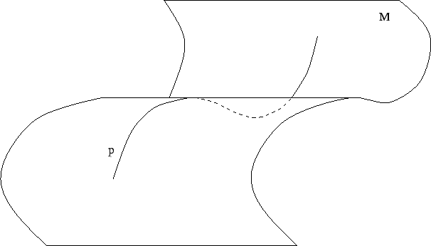
A result of Whitehead shows that for any point p there is a small region M surrounding it so that there is a unique geodesic in M joining any pair of points in M. The notion of between-ness is defined by saying that B lies between A and C in M if B lies on the (unique) geodesic joining A and C. Extending the geodesic within M beyond B and before A gives us the ``line'' joining A and B. We then easily check that Veblen's axioms of local geometry other than those involving planes are satisfied. In particular we have trouble verifying the Pasch axiom--numbered 7 in the list of Veblen's axioms given in section 1.
Let us therefore make the additional assumption that these axioms dealing with planes are satisfied; we will show that this imposes a restriction on the curvature of the Riemannian manifold M, which is satisfied if and only if M is a convex region in one of the ``classical'' geometries--Euclidean, Hyperbolic or Projective.
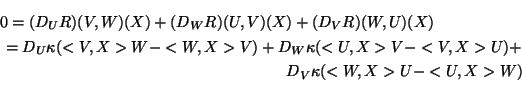
According to the results of section 1 we can choose coordinates on M in such a way that the geodesics are mapped into lines. In terms of these coordinates we see that a geodesic must be an accelerated path:
Now we have
![]() (X, Y)(p) =
(X, Y)(p) = ![]() (p) depends only on the point p.
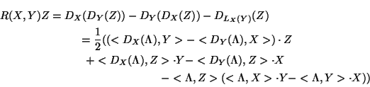
Thus we have
(p) depends only on the point p.
Thus we have