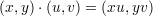
Other than addition and multiplication the first group that most high school students get introduced to is the group whose multiplication is defined by

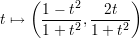
Consider the affine plane curve defined by the single equation X² + Y ² = 1; when (x,y) and (u,v) are points of this curve then the above rule defines a multiplication where (1,0) acts as identity. When the underlying field is , the field of real numbers, there are real numbers θ and ψ such that

In case you haven’t already recognised it, the above group law is recognisable as the addition law for sines and cosines. However, the above law makes sense over any field k. In fact, it works under the weaker hypothesis that X² + Y ² is non-zero; in other words it gives a group law on the points of the surface defined by Z(X² + Y ²) = 1. This can be used to show that if a and b are elements of the field that can each be written as the sum of two squares then so can their product.

The above is also the first interesting example of a group scheme or more specifically an affine algebraic group variety. We can write the equations (f_n(X,Y ),g_n(X,Y )) = (1,0) where f_n and g_n are polynomial expressions for the n-fold product (X,Y )(X,Y ). Since the original group law is commutative, these two equations also define an interesting finite group scheme—the corners of a regular polygon.

There is another more common (garden variety) of group scheme which is defined by the equation XY = 1 in the plane. For this the multiplication law is given by

This law points us in the direction in which we can look for more general group schemes.

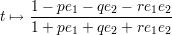
Let A be a k-algebra (which is associative but not necessarily commutative). Further assume that A is finite dimensional as a k vector space and let e₁, …, e_n be a basis such that e₁ = 1 is the identity element of A. In terms of this basis the multiplication law on A can be written as e_i ⋅ e_j = ∑ _kγ_ij^ke_k, or in other words

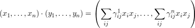
Consider the equations

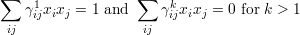
The equation of the hyperbola can be thought of as the special case of this equation for the case A = k. In general, this gives us an algebraic group which we denote by A^× and call the (algebraic) group of units of A.

In particular, we can think of the group of invertible n × n matrices. In this case the equations can be simplified a bit. We know that a matrix is invertible if and only if its determinant is non-zero; in fact, the inverse of a matrix A is (A^*)∕(det(A)), where A^*, the adjoint of A, is the matrix of (n - 1) × (n - 1) minors of A. Thus the above equation can be replaced with the equation det(A)T = 1, which is an equation in the entries A_ij of A and the supplemental variable T.

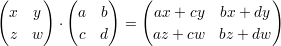
It is thus natural to define the group of 2 × 2 invertible matrices as the locus of solutions of the equation (XW -Y Z)T = 1. To simplify matters further, let us take matrices of determinant 1 which are given by the equation XW - Y Z = 1. Multiplication is given in the usual way

What is the sub-variety of this given by the equations X = W and Z = -Y ? Is it a group? (Hint: Look around).

More generally, the various matrix groups that we study are defined by algebraic equations; like AA^t = I for the orthogonal group. The study of these groups and algebraic group homomorphisms among them (which can be defined in an obvious way) goes under the name “linear algebraic groups and their representations”. It is a theorem that all affine algebraic groups are in fact linear algebraic groups.

Let us now look at a more exotic algebraic group which (unfortunately) most of you may not have encountered before. It was introduced by Hamilton to begin with but Clifford, Lipschitz, Grassmann and others developed it further. Somehow it is not in our mathematics syllabi but it is certainly in the physics syllabus!

Let us start again with the group of 2 × 2 matrices of determinant one given by the equation XW - Y Z = 1. Over the field of complex numbers (or any field where the equation T² + 1 = 0 has two distinct roots ±ι), this equation can be transformed (reversibly) into the equation A² + B² + C² + D² = 1 by means of the substitutions

Now, in terms of these new co-ordinates, the multiplication is given by

While this multiplication may look somewhat mysterious, it is not really so. Regard (x,y,z,w) as representing the quaternion x + yi + zj + wk, where i, j, k satisfy the rules i² = j² = k² = ijk = -1. We then see that the multiplication given above is the linear extension of these identities. It follows that the unit sphere of dimension 3 is also a group in a natural algebraic way. As before, the point (1,0,0,0) plays the role of identity. Moreover, we can again use this product rule to show that if a and b are each a sum of 4 squares, then so is the product ab.

Now consider the subspace of the three-dimensional sphere that consists of “purely imaginary” quaternions, i. e. quaternions of the form (0,b,c,d). This can be identified with the two-dimensional sphere. Moreover, this sub-variety of the quaternions is stable under the conjugation action of the quaternions on itself. The collection of all quaternions (x,y,z,w) that commute with (0,b,c,d) can be identified as (u,vb,vc,vd) where (u,v) is a point of the circle. It follows that we obtain the universal geometric identity S³∕S¹ = S².

How does one generalise the quaternions? One natural way (invented by Clifford) is to consider the k-algebra C_n (with unit) generated by e₁,…, e_n with the relations e_i² = -1 and e_ie_j = -e_je_i. When n = 2 we get the algebra of quaternions. We note that not every non-zero element of this algebra is invertible when n > 2; so we should further restrict our attention to the group C_n^× of units in C_n. However, this is also not enough for us as we also wish to generalise the action of C₂^× on the two-dimensional sphere. In terms of this description when n = 2, the subspace of imaginary quaternions is spanned by e₁, e₂ and e₁ ⋅e₂. A generalisation that suggests itself is to consider the subspace H of C_n which is spanned by the elements e_i and e_ie_j. We let Γ_n be the subgroup of C_n^× that preserves H under the conjugation action of this group on C_n. The group Γ_n is called the (non-normalised) spin group. There is a natural “norm” on C_n and the group Spin(n) is the subgroup of Γ_n that consists of elements of norm 1.

Let us return to the cases n = 1 and n = 2. There is a natural parametrisation of the circle x² + y² = 1 given by

In terms of the description of C₁ given above we note that

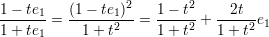
This suggests the parametrisation

for the unit quaternions in C₂. These parametrisations are due to Cayley and were generalised for C_n by R. Lipschitz who showed that the corresponding expression in that case indeed gives a parametrisation of Spin(n).

The study of the spin group and its representations is important for a lot of modern physics, geometry, analysis and number theory. Learn more about it as soon as possible! R. Sridharan, R. Parimala and their many students have undertaken an extensive study of quadratic forms over different kinds of fields using (among other things) the study of the associated Clifford algebra and algebraic groups. Many mathematicians such as M. S. Raghunathan have studied algebraic groups and associated number theoretic problems extensively.